[1] 0.001291758Medical Statistics
Important Probability Distributions
Boncho Ku, Ph.D. in Statistics 
Korea Institute of Oriental Medicine (KIOM)
Korea Institute of Oriental Medicine
Binomial Distribution
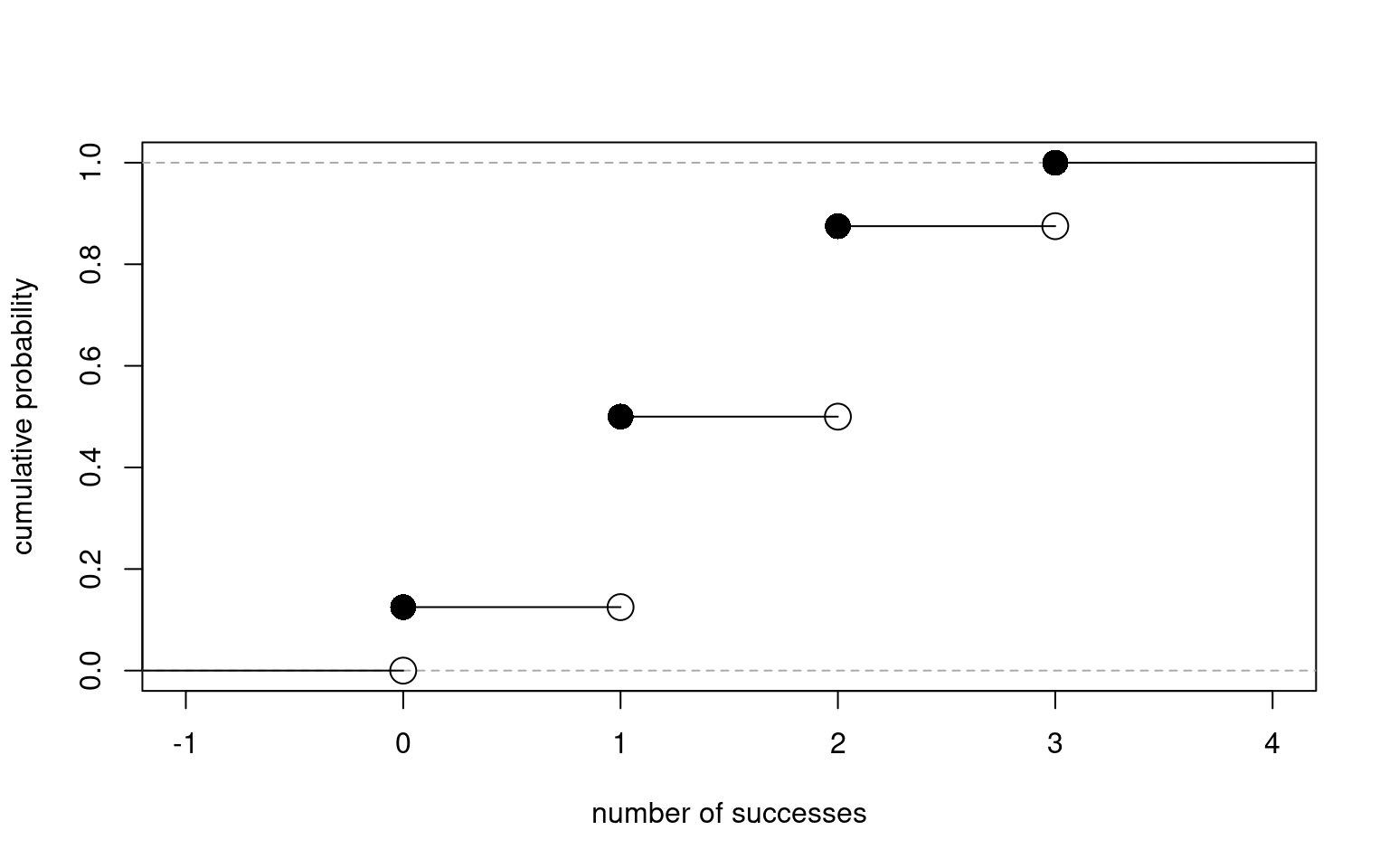
Example (CDF)
\[F_{X}(x) = P(X \leq x) = \begin{cases} 0, ~~~~~~~~~~~~~~~~~~~~~~x < 0\\ \frac{1}{8},~~~~~~~~~~~~~~~~~~~~~ 0\leq x < 1\\ \frac{1}{8} + \frac{3}{8} = \frac{4}{8},~~~~~ 1\leq x < 2\\ \frac{4}{8} + \frac{3}{8} = \frac{7}{8},~~~~~ 2\leq x < 3\\ 1 ~~~~~~~~~~~~~~~~~~~~~~~~x \geq 3\\ \end{cases}\]
n <- 3; p <- 0.5
x <- -1:(n+1)
y <- pbinom(x, size = n, p = p)

plot(x, y, type = "n",
     xlab = "number of successes",
     ylab = "cumulative probability")
abline(h=1, lty=2, col = "darkgray")
abline(h=0, lty=2, col = "darkgray")
points(x[2:5], y[2:5], pch=16, cex = 2)
points(x[2:5], y[1:4], pch=21, cex = 2)
segments(
  x0 = c(-2, 0, 1, 2, 3),
  x1 = c( 0, 1, 2, 3, 5),
  y0 = c(y[1], y[2], y[3], y[4], y[5]),
  y1 = c(y[1], y[2], y[3], y[4], y[5])
)
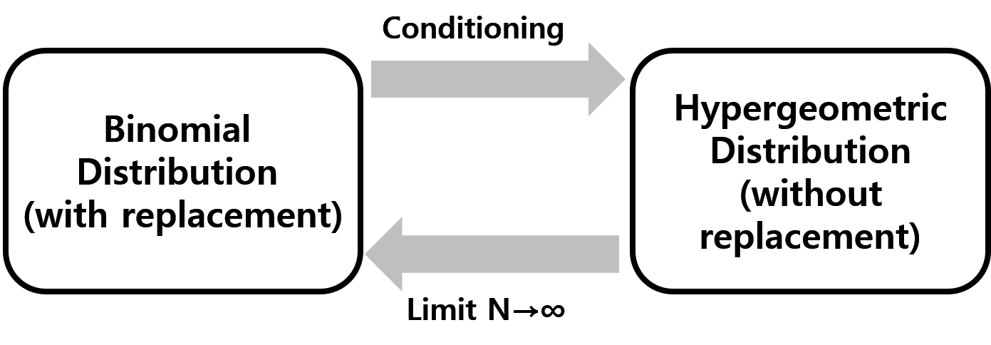
Hypergeometric Distribution
Relationship to Binomial Distribution
The conditional distribution of \(X\) given \(X+Y=K\) is identical to hypergeometric distribution.
When \(N \rightarrow \infty\), the hypergeometric distribution converges to the binomial distribution.
Important
Binomial distribution \(\rightarrow\) with replacement
Hypergeometric distribution \(\rightarrow\) without replacement
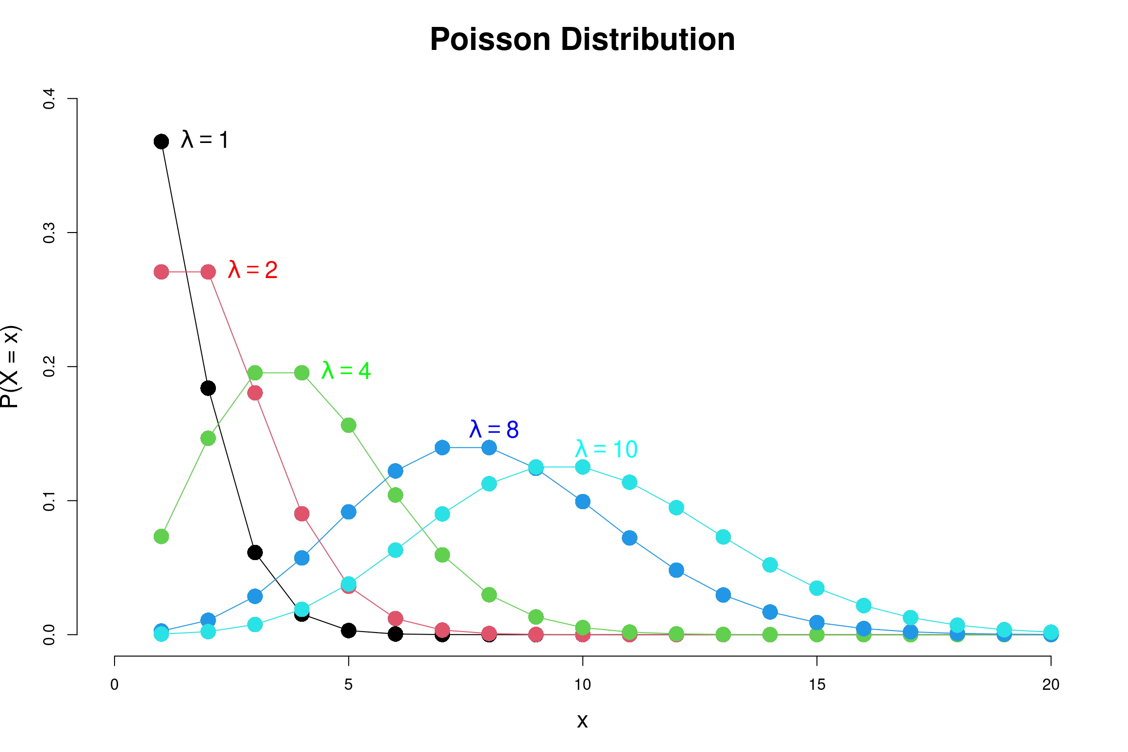
Poisson Distribution
\[E(X) = \sum_{x=0}^{\infty}x \frac{\lambda^x\exp(-\lambda)}{x!} = \sum_{x=0}^{\infty} \lambda \frac{\lambda^{(x-1)}\exp(-\lambda)}{(x-1)!} = \lambda\]
\[Var(X) = \sum_{x=0}^{\infty}x^2 \frac{\lambda^x\exp(-\lambda)}{x!} = \sum_{x=0}^{\infty} \lambda^2 \frac{\lambda^{(x-2)}\exp(-\lambda)}{(x-2)!} = \lambda^2\]
Shapes of Poisson Distribution according to \(\lambda\)
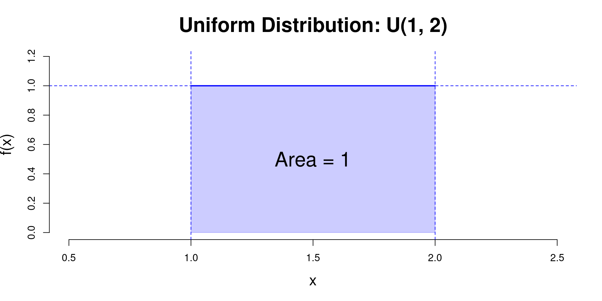
Uniform Distribution
Definition
When a random variable \(X\) with identical probability over every interval on \([a,b]\), it is called a uniform distribution
We write \(X \sim U(a, b)\) or \(X\sim \mathrm{unif}(\mathrm{min} = a, \mathrm{max}=b)\)
\[f_X(x) = \begin{cases} \frac{1}{b-a},~~ a\leq x \leq b \\ 0, ~~~~~~~ \mathrm{otherwise} \end{cases}\]
\[F_X(x) = \begin{cases} 0, ~~~~~~~ x < a\\ \frac{x-a}{b-a}, ~~ a\leq x \leq b\\ 1, ~~~~~~~ x > b \end{cases}\]
\[\begin{aligned} \mu_X = E(X) &= \int_{-\infty}^{\infty} x f_X(x) dx \\ &= \int_{a}^{b} x \frac{1}{b-a} dx \\ &= \frac{1}{b-a}\frac{x^2}{2} \bigg|_{x=a}^{b} \\ &= \frac{b+a}{2} \end{aligned}\]
\[\begin{aligned} \sigma^2_X &= Var(X) = E\left[(X - E(X))^2\right] = E(X^2) - \left[E(X)\right]^2 \\ &= \int_{a}^{b} x^2 \frac{1}{b-a} dx - \left(\frac{b+a}{2}\right)^2 \\ &= \frac{1}{b-a}\frac{x^3}{3}\bigg|_{x=a}^{b} - \left(\frac{b+a}{2}\right)^2 = \frac{b^3-a^3}{3(b-a)} - \left(\frac{b+a}{2}\right)^2\\ &= \frac{(b-a)^2}{12} \end{aligned}\]
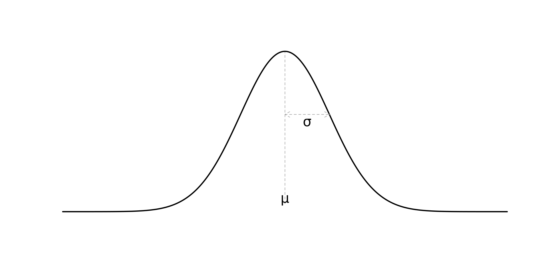
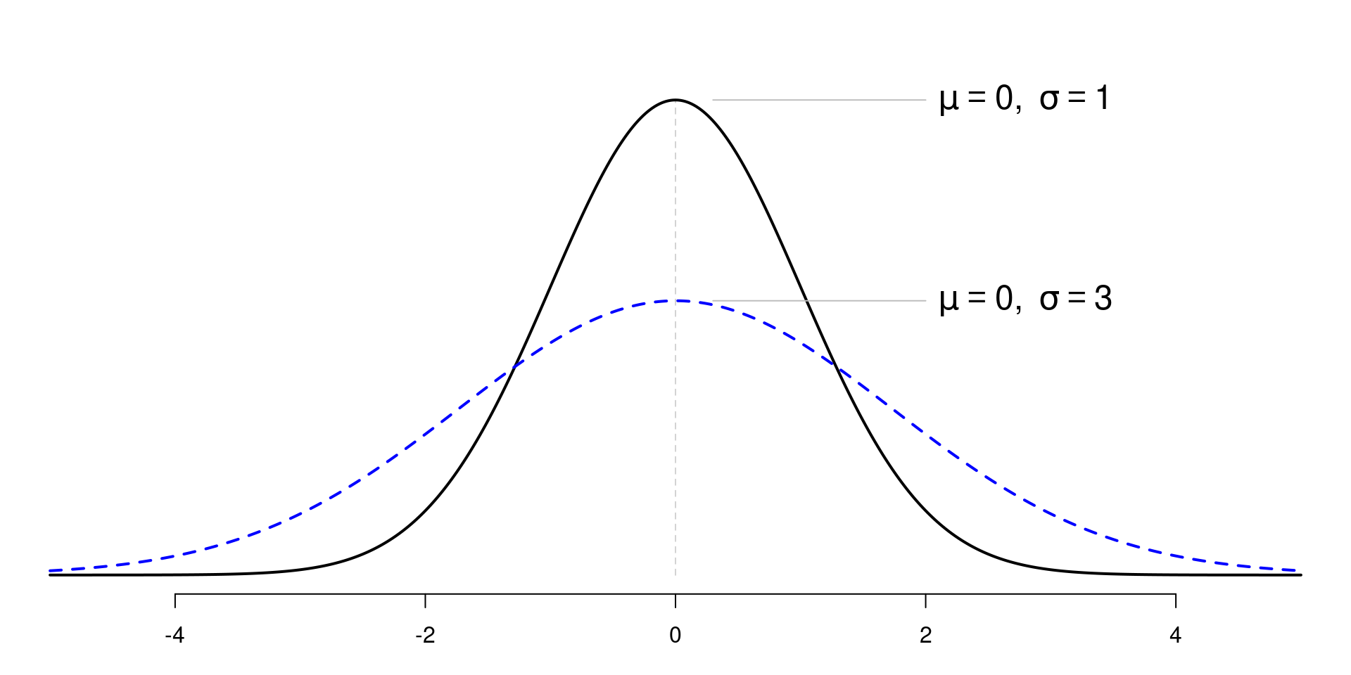
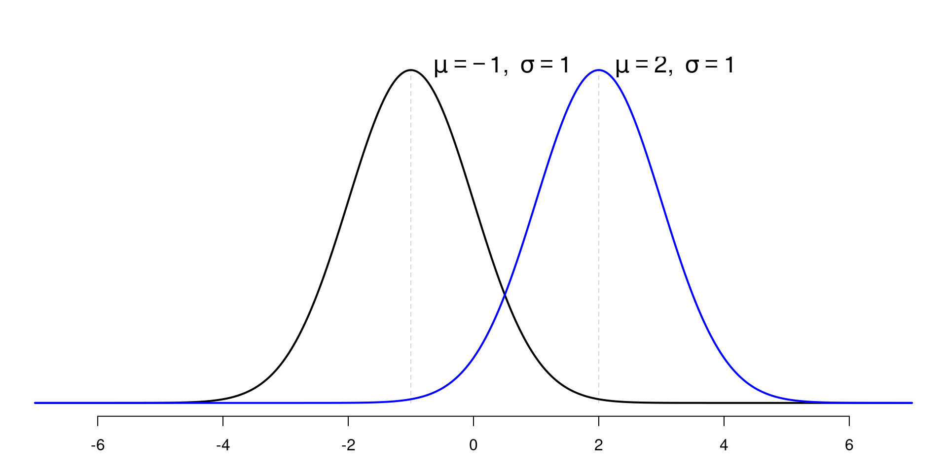
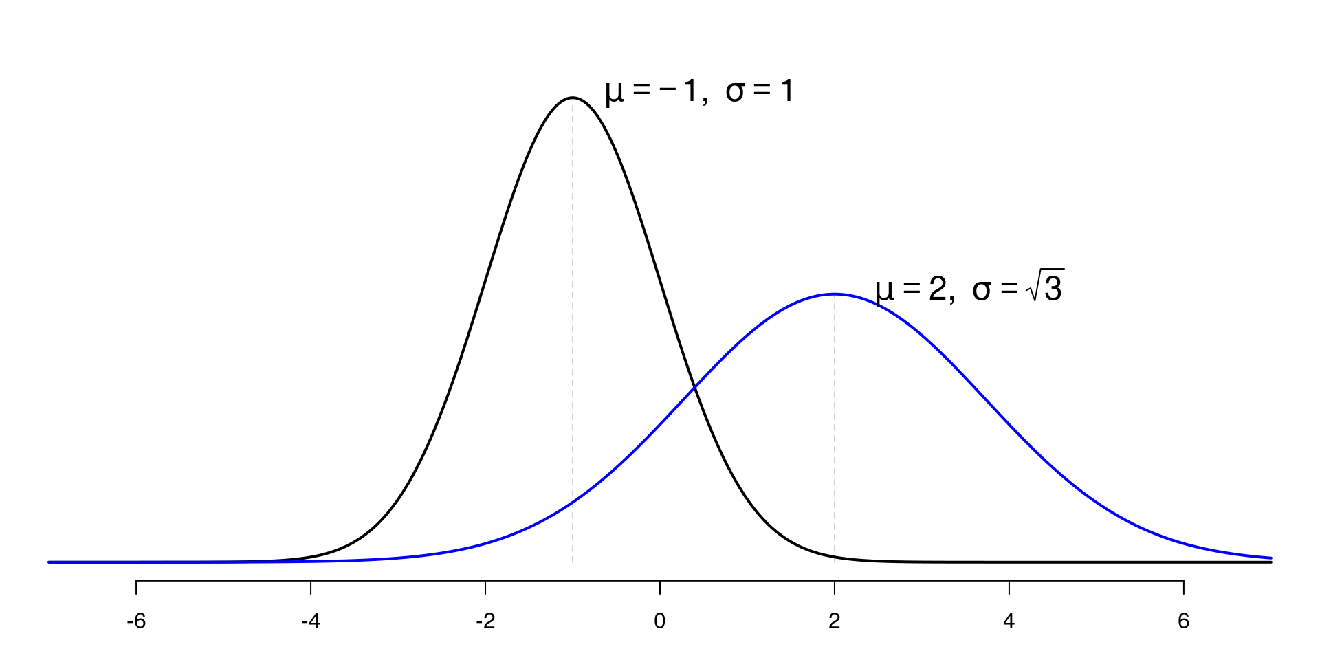
Normal Distribution
Shapes
- Bell shaped curve and symmetric around the \(\mu\)
- mean = median = mode
- Depends on \(\mu\) and \(\sigma\)
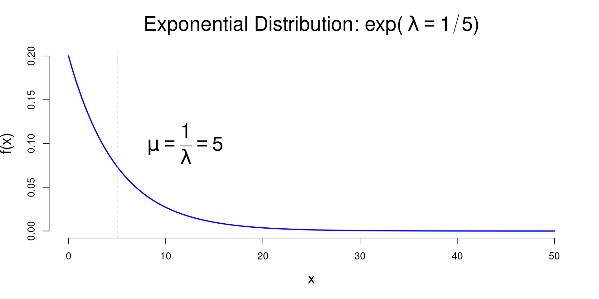
Exponential DIstribution
Definition
A random variable \(X\) has an exponential distribution and write \(X \sim \exp(\lambda)\)
\[ f_X(x) = \lambda \exp(-\lambda x),~~~~x\geq0 \] where
- \(x\): The time until the next event occurs;
- \(\lambda\): The rate at which events occur
\[ F_X(x) = 1 - \exp(-\lambda x),~~~~x\geq0 \]
\[\begin{aligned} \mu_X &=E(X) = \frac{1}{\lambda} \\ \sigma^2_X &= Var(X) = \frac{1}{\lambda^{2}} \end{aligned}\]
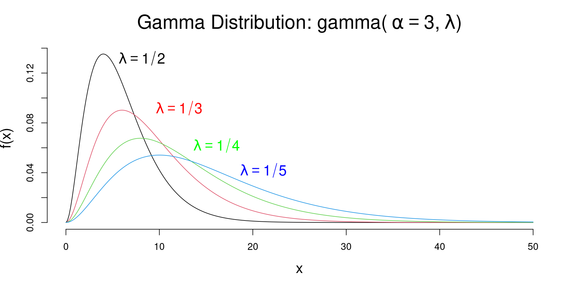
Gamma Distribution
Definition
A generalization of the exponential distribution. A random variable \(X\) is said to have a gamma distribution with shape parameter \(\alpha\) and inverse scale parameter (shape) \(\lambda = 1/\theta\), denoted as \(X \sim \mathrm{gamma}(\alpha, \lambda)\)
Parameterized by shape \(\alpha\) and inverse scale \(\lambda\)
\[ f_X(x; \alpha, \lambda) = \frac{\lambda^\alpha}{\Gamma(\alpha)}x^{\alpha - 1}\exp(-\lambda x),~~ x>0 \] where
- \(\Gamma(\alpha)\) is the gamma function defined as \(\Gamma(\alpha) = (\alpha - 1)!\)
Parameterized by shape \(\alpha\) and scale \(\theta\)
\[ f_X(x; \alpha, \theta) = \frac{1}{\Gamma(\alpha)\theta^\alpha}x^{\alpha - 1}\exp\left(-\frac{x}{\theta}\right),~~ x>0 \]
Parameterized by shape \(\alpha\) and inverse scale \(\lambda\)
\[\begin{aligned} \mu_X &=E(X) = \frac{\alpha}{\lambda} \\ \sigma^2_X &= Var(X) = \frac{\alpha}{\lambda^{2}} \end{aligned}\]
Parameterized by shape \(\alpha\) and scale \(\theta\)
\[\begin{aligned} \mu_X &=E(X) = \alpha \theta \\ \sigma^2_X &= Var(X) = \alpha \theta^{2} \end{aligned}\]
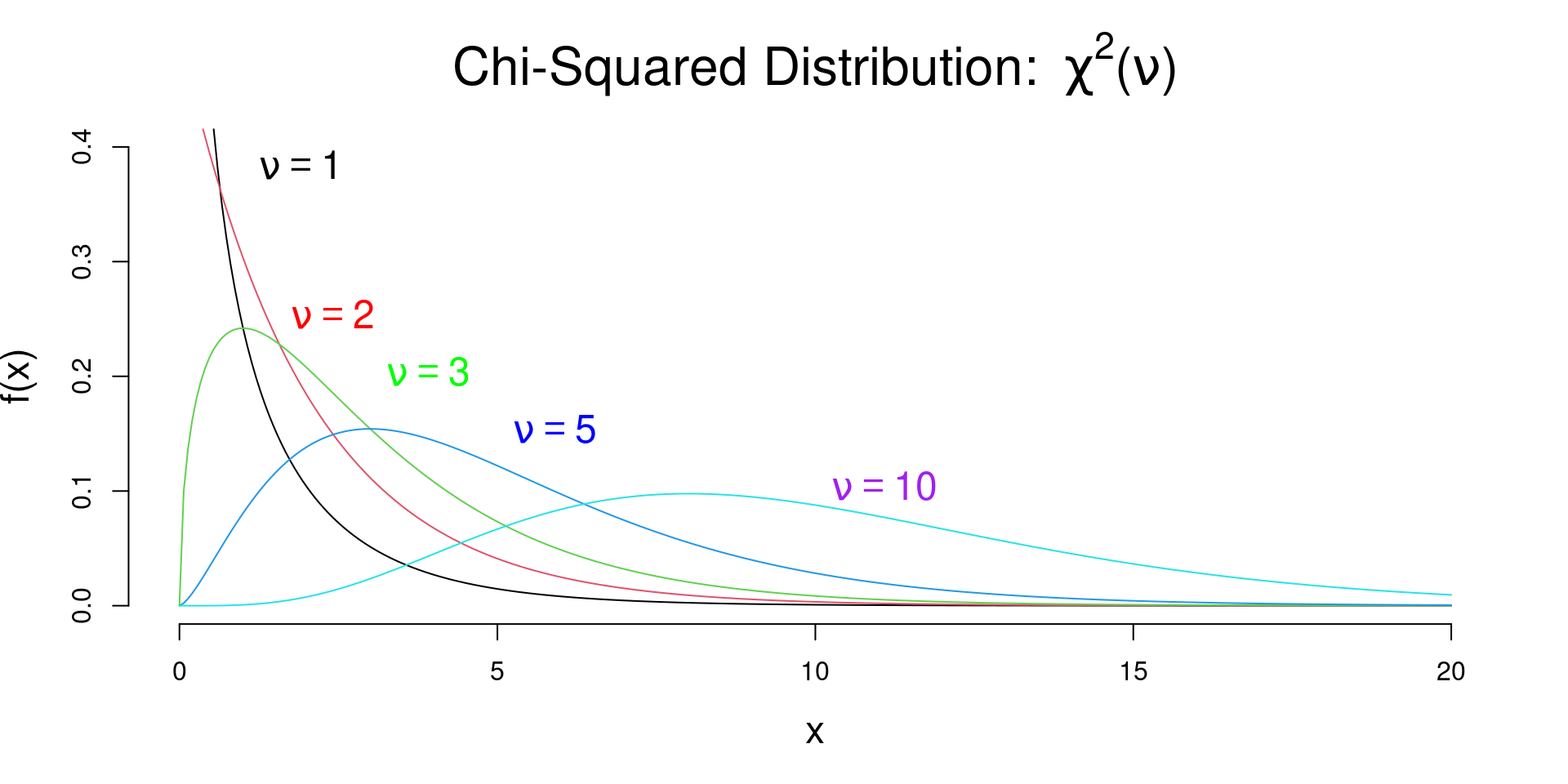
\(\chi^2\) Distribution
Definition
A random variable \(X\) is said to have a chi-square distribution with \(\nu\) degrees of freedom, denoted as \(X \sim \chi^2(\nu)\)
\[f_X(x; \nu) = \frac{1}{\Gamma\left(\nu/2\right)2^{\nu/2}}x^{\nu/2-1}\exp[-x/2],~~x\geq 0\]
where \(\nu > 0\) is the degrees of freedom (integer),
\[ \Gamma(\nu/2) = \int_{0}^{\infty} t^{\nu/2-1}\exp(-t) dt,~~ z>0 \]
\[\begin{aligned} \mu_X &=E(X) = \nu \\ \sigma^2_X &= Var(X) = 2\nu \end{aligned}\]
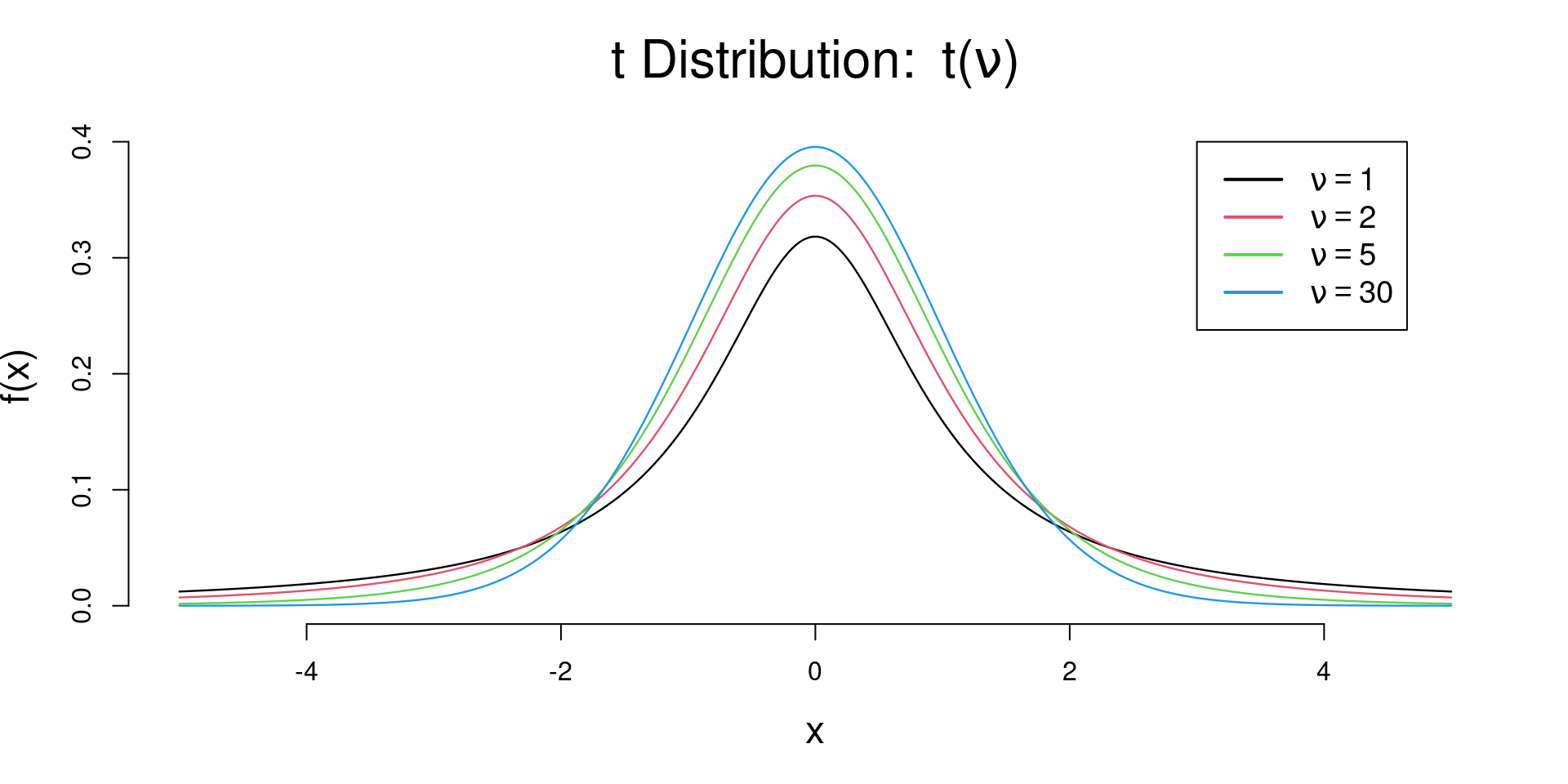
t Distribution
Definition
A random variable \(X\) is said to have a \(t\) distribution with \(\nu\) degrees of freedom, denoted as \(X \sim t(\nu)\)
\[f_X(x; \nu) = \frac{\Gamma\left[ (r+1)/2 \right ]}{\sqrt{\nu\pi}\Gamma(\nu/2)} \left (1 + \frac{x^2}{r} \right )^{-(\nu+1)/2}, ~~~~~ -\infty < x < \infty\]
where \(\nu > 1\) is the degrees of freedom (integer) and \(\Gamma(\cdot)\) is the gamma function.
\[\begin{aligned} \mu_X &=E(X) = 0, ~~ \nu > 1 \\ \sigma^2_X &= Var(X) = \frac{\nu}{\nu - 2}, ~~ \nu > 2 \end{aligned}\]
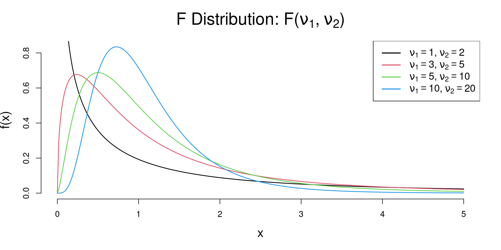
F Distribution
Definition
A random variable \(X\) is said to have a \(F\) distribution with \((\nu_1, \nu_2)\) degrees of freedom, denoted as \(X \sim F(\nu_1, \nu_2)\)
\[f_X(x; \nu_1, \nu_2) = \frac{\Gamma\left(\frac{\nu_1 + \nu_2}{2}\right)}{\Gamma\left(\frac{\nu_1}{2}\right)\Gamma\left(\frac{\nu_2}{2}\right)}\left(\frac{\nu_1}{\nu_2}\right)^{\nu_1/2} \frac{x^{\nu_1/2 - 1}}{\left(1 + \frac{\nu_1}{\nu_2}x\right)^{(\nu_1 + \nu_2)/2}},~~ x\geq 0\]
where \(\nu_1\) and \(\nu_2\) are the degrees of freedom (integers) and \(\Gamma(\cdot)\) is the gamma function.
\[\begin{aligned} \mu_X &=E(X) = \frac{\nu_2}{\nu_2 - 2}, ~~ \nu_2 > 2 \\ \sigma^2_X &= Var(X) = \frac{2\nu_2^2(\nu_1 + \nu_2 - 2)}{\nu_1(\nu_2 - 2)^2(\nu_2 - 4)}, ~~ \nu_2 > 4 \end{aligned}\]
F Distribution
Properties (Continued)
- Application:
- The F-distribution is commonly used in analysis of variance (ANOVA) to compare the variances of two or more groups.
- It is also used in regression analysis to test the overall significance of a regression model.
Let \(X_1\ldots X_n \overset{i.i.d}{\sim} N(\mu_1, \sigma^2_1)\), \(Y_1\ldots Y_m \overset{i.i.d}{\sim} N(\mu_2, \sigma^2_2)\), and sample variances \(S^2_X=\sum_{i=1}^{n}(X_i - \bar{X})^2/(n-1)\), \(S^2_Y=\sum_{j=1}^{m}(Y_j - \bar{Y})^2/(m-1)\), then
\[ \frac{S^2_X/\sigma^2_1}{S^2_Y/\sigma^2_2} \sim F(n-1, m-1) \]